The development of modern industrial technology has driven continuous progress in the automotive manufacturing industry. Therefore, the processing accuracy and efficiency of automotive components have become key research priorities.
CNC milling machines play an increasingly vital role in modern automotive parts manufacturing.
However, current CNC milling machines lack the positioning accuracy needed for high-precision automotive parts.
Therefore, improving CNC milling positioning accuracy is crucial for enhancing automotive parts quality and production efficiency.
In modern automotive manufacturing, component precision directly affects vehicle performance and quality.
For example, engine parts, transmission gears, and suspension components require high precision to ensure stability and reliability.
CNC milling of high-precision parts often faces positioning and thermal deformation errors, leading to parts that don’t meet design specs.
This not only affects vehicle performance and quality but also increases production costs and the complexity of post-production maintenance.
Technicians are improving CNC milling accuracy through design, processes, control, and error compensation.
High-performance servo drives and advanced algorithms improve control precision, reducing positioning and dynamic errors.
However, based on the phased implementation progress of related work, most of these technologies have limitations in practical application.
This paper studies methods to improve positioning accuracy using CNC milling of a specific automotive part as an example.
Feature Point Extraction of Automotive Parts Processed by CNC Milling Machines Based on Point Cloud Data
CNC milling machines precisely cut metal automatically for automotive parts manufacturing.
Imagine it as a highly stable mechanical arm capable of carving complex parts along predefined paths.
However, to achieve both speed and accuracy in processing, there is a prerequisite:
We must first accurately know the shape and features of each position of the part.
This is like knowing where each point is before drawing, so as not to draw incorrectly.
To achieve this, we first use a scanner to convert the part’s shape into 3D point cloud data.
A point cloud is a set of points representing an object’s surface positions.
When viewed as a whole, it resembles a 3D model composed of countless minor points.
This collection of points is denoted as:
Q={qi, i = 1, 2, …, n}
This means we have n points, where each qi is a three-dimensional coordinate point representing the x, y, and z values of a specific location.
However, the original process places these points in a disordered and random arrangement, like someone scattering a pile of paper scraps on a table.
To identify feature points like edges or corners, we first find each point’s neighbors.
How do we find neighbors? We use a technique called the k-nearest neighbor method.
For each point qi, we find the k nearest points to it and form a “neighbor set” called Vqi.
However, these neighbors must satisfy one condition: they cannot be too far from the main point:
‖qi– vj‖<r. (1)
Here, vj is one of qi‘s neighbors, vj ∈Vqi, and vj ≠qi represents the distance between two points, and r is a range radius that we set ourselves.
This is like only recognizing “neighbors within a radius of r meters” and not considering those beyond that range as “acquaintances.”
Neighbors connect each point to its surroundings, forming a topological relationship.
Next, we will determine whether a point is a feature point based on the “surface curvature” around each point.
Put: if the surface around a point does not change much, it is likely a flat area.
If the changes are drastic, such as sudden turns, corners, or edges, it is likely an important “feature point.”
“Surface change degree” helps filter key points from the point set for processing.
Next, we need to determine whether each point is a “feature point” using a method called “surface change degree.”
Imagine you spread out a piece of fabric. In some places it is flat, while in others there are wrinkles or protrusions.
We want to identify those areas with noticeable changes that are not entirely flat.
For point clouds, we often focus on these “noticeably changing” areas as the feature points.
How do we determine the extent of the change? We use a mathematical tool called “covariance analysis.”
Step 1: Calculate the covariance matrix
Starting from point qi, we examine its m neighbors found by the k-nearest neighbor algorithm.
Then we calculate the “covariance matrix” of these points, denoted as:

This can be broken down as follows:
̅v is the mean of the points in the neighborhood of qi;
By analyzing the differences between each neighboring point and the central point, we can observe how these points are distributed in space.
This covariance matrix ultimately produces three numbers called eigenvalues (λ1, λ2, λ3, where λ1 ≤ λ2 ≤ λ3).
These three numbers tell us how much the points in this small area vary in three directions.
The largest λ3 indicates normal variation, or “curvature,” which increases with surface undulation.
Step 2: Calculate the curvature estimate
To make this degree of variation more concrete, we define a “curvature estimate,” denoted as δi:
δi = λ3{λ1 + λ2 + λ3} (3)
This value tells us: how much of the total change at this point is due to “curvature.”
If a point is in a flat area, λ3 will be smaller, so δi will be small;if it is a protrusion or sharp corner, λ3 will be larger, and δi will also be larger.
Since λ are all non-negative, the value of δi must be between 0 and 1.
Step 3: Set the threshold value
A set of δi values alone isn’t enough; points above a threshold are identified as features.
This threshold value is denoted as θ and is calculated as follows:
θ = αδavg + (1 – α)δmax (4)
This formula means:δavg: the average curvature of all points;δmax: the maximum curvature value;
α: a control parameter (e.g., 0.5 represents equal weighting between the average and maximum values).
This approach allows us to flexibly determine the judgment criteria, avoiding being too strict or too lenient.
Step 4: Perform feature point detection
Finally, we define a simple “detection rule” to determine whether a point is a feature point, represented by a symbol function φ(qi):
φ(qi) = 1, if δi >=θ
Or
φ(qi) = 0, otherwise
Meaning:
If the curvature of this point is greater than or equal to the threshold value we set, it is marked as a feature point (value is 1);
Otherwise, it is not a feature point (value is 0). These steps accurately identify shape feature points from the chaotic point cloud.
These points guide CNC milling for precise, high-quality parts.
CNC Milling Machine Processing Error Modeling
During the process of machining automotive parts using a CNC milling machine, errors are inevitable.
These errors cause slight part deviations, affecting quality like a shaky hand distorts a line.
We can analyze error sources and impacts, then design methods to reduce them.
This requires establishing a mathematical model of the errors.
Sources of machining errors: from tools and workpieces
We know that errors primarily come from two sources:
● Tool position error: simply put, this refers to the milling cutter itself moving inaccurately, denoted as ΔP
●Workpiece positioning error: This refers to slight deviations in the position of the metal part, denoted as ΔW
Therefore, the machining error ΔE is the sum of these two errors.
However, these errors only occur at the feature points of interest, so the formula is written as:
ΔE = φ(qi)(ΔP + ΔW) (6)
Here, φ(qi) is the feature point determination function (as mentioned earlier, if it is a feature point, it equals 1; otherwise, it equals 0).
Describing the direction of error using vectors
Error is not just about magnitude; it also has a direction — for example, a point may be offset by 0.1 mm to the right and 0.2 mm upward.
We use a three-dimensional vector to represent this offset, called the error vector ΔvecE, with the following formula:
![]() = (Δxi, Δzi, Δzi)/ΔE (7)
= (Δxi, Δzi, Δzi)/ΔE (7)
Where:
●Δxi, Δzi, Δzi are the displacement amounts of the feature point in the three directions before and after processing;
●Division by ΔE is to “normalize” this vector, so it only represents direction and not magnitude.
Overall Error Assessment Model
Now that we know the error vector for each point, we also want to know the overall processing error.
At this point, we use the formula (8) in the figure:

Where: R is the error model; N is the number of feature points quantified.
Through the above steps, the error modeling for CNC milling machine processing is completed.
This formula calculates the average spatial displacement of all feature points in three directions.
● It tells us: “On average, how much has each important point deviated after machining?”
This quantification method helps engineers quickly assess machining quality and determine whether the machine needs adjustment.
To summarize, the process of this model is:
Start from tool and workpiece errors → obtain the overall machining error ΔE;
Represent the error direction of each point using vectors.
Sum and average the offsets of all feature points → obtain the overall machining deviation R.
This lets us identify issues and improve CNC milling precision by addressing hidden machining errors.
Improving Positioning Accuracy Based on Tool Path Control
Earlier, we modeled processing errors, measured each feature point’s deviation (error vector ![]() ), and calculated total error R.
), and calculated total error R.
Next, we proactively compensate for deviations—like steering left to counter a rightward wind—to ensure perfect alignment.
This is what we refer to as tool path compensation design.
Adjusted tool path: error compensation
We originally had a tool movement path T(t), representing the position the tool should be at time t.
Now we add a compensation vector to slightly deviate from the original path, thereby offsetting the error.
The formula for the new path after compensation is as follows:
T'(t) = T(t) + ![]() (t) * (R –
(t) * (R – ![]() ) (9)
) (9)
The meaning of each term is as follows:
●T(t): The original tool trajectory;
●T'(t): The adjusted tool trajectory (what we want);
●![]() : The compensation vector, which is a direction and proportion calculated based on the error;
: The compensation vector, which is a direction and proportion calculated based on the error;
●R: The overall average error;
●![]() : The actual observed error vector.
: The actual observed error vector.
This formula calculates compensation by comparing the expected error (R) with the actual offset (![]() ) and adjusts the tool path accordingly.
) and adjusts the tool path accordingly.
In other words, we make the tool move in such a way that it exactly offsets the error.
Why isn’t the compensation vector ![]() (t) fixed?
(t) fixed?
In machining, multiple feature points exist, each with varying error directions and magnitudes.
Therefore, the compensation vector ![]() (t) is determined by considering the errors of all points comprehensively.
(t) is determined by considering the errors of all points comprehensively.
It can be understood as a “comprehensive adjustment plan.”
Practical application: correction during machining
In actual machining, we can have the machine adjust the tool path according to this formula while machining.
After machining a few points, we update T(t) to the new T'(t) based on the newly measured error.
This method is dynamic and iterative — just like GPS continuously adjusts the navigation direction based on your current position and deviation.
Through continuous adjustment and optimization, we can:
● Effectively reduce processing errors;
● Significantly improve positioning accuracy;
● Combine with other technologies (such as thermal error control) to further enhance overall accuracy.
In summary, the core idea here is: “I know you will make mistakes so that I will compensate for them in advance.”
This intelligent compensation makes CNC milling more stable and accurate, producing higher-quality automotive parts.
Case Study Analysis
Experimental Preparation
This experiment used a regional automotive parts facility with advanced CNC milling machines for precision processing.
Preliminary data show CNC milling machines at the facility have over 85% utilization, highlighting their production role.
The facility maintains ±0.05mm processing errors using precise tools and optimized tool paths, improving accuracy and surface quality.
Table 1 below shows an analysis of the technical parameters of CNC milling machine processing for automotive parts at the pilot unit.

To improve CNC milling positioning accuracy, the machine underwent thorough inspection and calibration to optimize performance.
The team arranged the processing area to minimize positioning errors of workpieces, fixtures, and tools.
High-precision instruments monitored key parameters in real-time during machining.
Experts collected and analyzed data to ensure accurate, reliable experimental results.
Through the steps above, the team completed experimental preparation and related tasks.
Visual Inspection of Tool Trajectories in CNC Milling Machine Processing of Automotive Parts
Visual inspection of tool paths is key to improving CNC milling positioning accuracy.
Visualization lets technicians monitor tool paths in real time, quickly spotting and correcting errors for precise machining.
Experiments compare expected and actual tool paths to accurately assess positioning errors, guiding error compensation.
During inspection, technicians use visualization software to import tool trajectory data for simulation and analysis.
High-precision instruments monitor and record tool trajectories in real-time during machining.
By comparing the simulation results with the actual data, we evaluate the reliability of the design method.
The results are shown in Figure 1.

In CNC milling machine processing of automotive parts, visualization inspection of tool trajectories is critical for ensuring processing accuracy.
The experiment showed high consistency between expected and actual tool paths, proving the method’s practical feasibility.
Figure 1 shows the tool closely follows the designed path with minimal positioning error after applying this method.
This result verifies the method’s accuracy and supports future CNC machining of automotive parts.
Visual inspection lets technicians quickly spot and fix errors, ensuring stable, consistent processing quality.
Inspection of positioning accuracy in CNC milling machine processing of automotive parts
Based on the above content, we inspected positioning accuracy in the CNC milling machine processing of automotive parts.
This method extracted and matched spatial scatter points with the designed layout.
High compatibility shows that it improves CNC milling positioning accuracy.
Low compatibility indicates poor positioning accuracy of the method in CNC milling applications.
Based on this, we analyze the experimental results, as shown in Figures 2 and 3.
As shown in Figures 2 and 3, the scatter distribution of processed automotive parts exhibits high compatibility with the designed planar distribution.
This result shows the method significantly improves CNC milling positioning accuracy for automotive parts.
The high match between scatter and design verifies the method’s accuracy and supports precise automotive part processing.
This method ensures high-quality, precise automotive parts production.


Conclusion
Improving CNC milling positioning accuracy is vital for better quality and efficiency in automotive parts production.
This research boosts machine tool positioning accuracy, supporting modern automotive manufacturing.
This method uses point cloud features and error modeling to enhance CNC machining accuracy.
The proposed design improves positioning accuracy by precisely controlling the tool path, minimizing errors, and ensuring trajectory consistency.
Visualization technology enables technicians to monitor tool movement, quickly identify and correct errors, ensuring stable, consistent quality.
In summary, this method offers strong technical support for automotive parts production.